
Slika:Lemniscates5.png

Izvorna datoteka (1.000 × 1.000 točk, velikost datoteke: 73 KB, MIME-vrsta: image/png)
Spodaj prikazane informacije so s tamkajšnje opisne strani.

|
To grafiko je mogoče poustvariti z uporabo vektorske grafike kot SVG-datoteko. To ima več prednosti; več informacij je na razpolago na strani Commons:Media for cleanup. Če je SVG-oblika te datoteke že na razpolago, jo, prosimo, naložite. Potem, ko boste SVG naložili, to predlogo zamenjajte z izrazom {{vector version available|ime nove slike.svg}}.
|
Povzetek
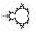
| Opis | 6 lemniscates of Mandelbrot set. Computed using implicit equations. |
| Vir | self-made with help of many people, using free CAS Maxima, Gnuplot and implicit_plot package (by Andrej Vodopivec) |
| Avtor | Adam majewski |
| Druge različice | lemniscates for Julia set |
Compare with
-
 DEM and sobel
 -
 LCM/J; ER=1000
 -
 LCM/J but better algorithm, ER = 2
 -
 LSM/J B&W; ER = 1000
 -
 LSM/J colour ( probably made with Fractint ); ER = 2


See also:
Long description
" instead of iterating a point through a nice fractal-generating function until it exits the containing circle, I'm starting with the containing circle's function (2cos(t),2sin(t)) and iterating that circle function through the inverse of the fractal-generating function." Axis Angels[1]
Few lemniscates of Mandelbrot set[2]. They are boundaries of Level Sets of escape time ( LSM/M [3]).
They are in parameter plane (c-plane, complex plane ).
Definition :

where
is Escape Radius, bailout value, radius of circle which is used to measure if orbit of is bounded; it is integer number


are complex numbers (points of 2-D planes )

is point of dynamical plane ( z-plane)

is point of parameter plane ( c-plane)


One can compute first few iterations :


and so on .
Then :


...
is a circle,

is an Cassini oval,


These curves tend to boundary of Mandelbrot set as n goes to infinity.
If ER < 2 they are inside Mandelbrot set[6].
If ER = 2 curves meet together ( have common point) c = −2. Thus they can't be equipotential lines.
If ER ≥ 2 they are outside of Mandelbrot set. They can also be drawn using Level Curves Method.
If ER >> 2 they aproximate equipotential lines ( level curves of real potential , see CPM/M ).
Maxima source code
 /* based on the code by Jaime Villate */
 load(implicit_plot); /* package by Andrej Vodopivec */

 c: x+%i*y;

 ER:2; /* Escape Radius = bailout value it should be >=2 */

 f[n](c) := if n=1 then c else (f[n-1](c)^2 + c);

 ip_grid:[100,100];  /* sets the grid for the first sampling in implicit plots. Default value: [50, 50] */
 ip_grid_in:[15,15]; /* sets the grid for the second sampling in implicit plots. Default value: [5, 5] */

 my_preamble: "set zeroaxis; set title 'Boundaries of level sets of escape time of Mandelbrot set'; set xlabel 'Re(c)';  set ylabel 'Im(c)'";

 implicit_plot(makelist(abs(ev(f[n](c)))=ER,n,1,6), [x,-2.5,2.5],[y,-2.5,2.5],[gnuplot_preamble, my_preamble],
 [gnuplot_term,"png   size  1000,1000"],[gnuplot_out_file, "lemniscates6.png"]);
For curves 1-5 it works, but for curve number 6 this program fails( also Mathematica program[7]), because of floating point error.
One have to change the method of computing lemniscates . Here is the code and explanation by Andrej Vodopivec" "You can trick implicit_plot to do computations in higher precision. Implicit_draw will draw the boundary of the region where the function has negative value. You can define a function f6 which computes the sign of f[6] using bigfloats and then plot f6."
/* based on the code by Jaime Villate and Andrej Vodopivec*/
c: x+%i*y;
ER:2;
f[n](c) := if n=1 then c else (f[n-1](c)^2 + c);
F(x,y):=block([x:bfloat(x), y:bfloat(y)],if abs((f[6](c)))>ER then 1 else -1);
fpprec:32;
load(implicit_plot); /* package by Andrej Vodopivec */
ip_grid:[100,100];
ip_grid_in:[15,15];
implicit_plot(append(makelist(abs(ev(f[n](c)))=ER,n,1,5), ['(F(x,y))]),[x,-2.5,2.5],[y,-2.5,2.5]);
Questions
- What is mathemathical description of these curves ?
Rerferences
- ↑ You tube video
- ↑ lemniscates at Mandelbrot Set Glossary and Encyclopedia, by Robert Munafo
- ↑ LSM/M
- ↑ Weisstein, Eric W. "Pear Curve." From MathWorld--A Wolfram Web Resource. http://mathworld.wolfram.com/PearCurve.html
- ↑ Mandelbrot lemniscate at 2DCurves by Jan Wassenaar
- ↑ Polynomial_lemniscate
- ↑ | Weisstein, Eric W. "Mandelbrot Set Lemniscate." From MathWorld--A Wolfram Web Resource.
Licenca

|
Ta dokument je dovoljeno kopirati, razširjati in/ali spreminjati pod pogoji Licence GNU za prosto dokumentacijo, različica 1.2 ali katera koli poznejša, ki jo je objavila ustanova Free Software Foundation; brez nespremenljivih delov ter brez besedil na sprednji ali zadnji platnici. Kopija licence je vključena v razdelek Licenca GNU za prosto dokumentacijo. |
- Dovoljeno vam je:
- deljenje – reproducirati, distribuirati in javno priobčevati delo
- predelava – predelati delo
- Pod naslednjimi pogoji:
- priznanje avtorstva – Navesti morate ustrezno avtorstvo, povezavo do licence in morebitne spremembe. To lahko storite na kakršen koli primeren način, vendar ne na način, ki bi nakazoval, da dajalec licence podpira vas ali vašo uporabo dela.
- deljenje pod enakimi pogoji – Če boste to vsebino predelali, preoblikovali ali uporabili kot izhodišče za drugo delo, morate svoj prispevek distribuirati pod enako ali združljivo licenco, kot jo ima izvirnik.
Zgodovina datoteke
Kliknite datum in čas za ogled datoteke, ki je bila takrat naložena.
| Datum in čas | Sličica | Velikost | Uporabnik | Komentar | |
|---|---|---|---|---|---|
| trenutno | 21:42, 11. januar 2009 | | 1.000 × 1.000 (73 KB) | Geek3 | smooth and precise plotcurve |
| 12:22, 18. marec 2008 |  | 1.000 × 1.000 (17 KB) | Soul windsurfer | added 6 lemniscate | |
| 10:15, 16. marec 2008 |  | 1.000 × 1.000 (15 KB) | Soul windsurfer | {{Information |Description= |Source=self-made |Date= |Author= Adam majewski |Permission= |other_versions= }} |
Uporaba datoteke
Datoteka je del naslednje 1 strani slovenske Wikipedije (strani drugih projektov niso navedene):
Globalna uporaba datoteke
To datoteko uporabljajo tudi naslednji vikiji:
- Uporaba na ca.wikipedia.org
- Uporaba na en.wikibooks.org